
In aqueous solutions, bases bind protons, while acids dissociate them. For weak acids and bases, these protonation reactions occur in the intermediate pH range. Dealing with monoprotic or diprotic acids and bases, the corresponding binding isotherm is referred to as the titration curve, and the corresponding chemical equilibria are discussed in all introductory chemistry courses.
When one is interested in the binding of protons to weak polyelectrolytes, the situation is more complicated. The principal reason is that in polyelectrolytes many ionizable sites interact and the binding isotherm is the result of the many-body interactions among all of them. For a monoprotic acid or base, there is only one site, and interactions play no role. For a diprotic system, interactions start to play a role, but can be treated within the classical chemical equilibrium framework. Here we explain how to describe and to understand the titration curves of weak polyelectrolytes [1,2].
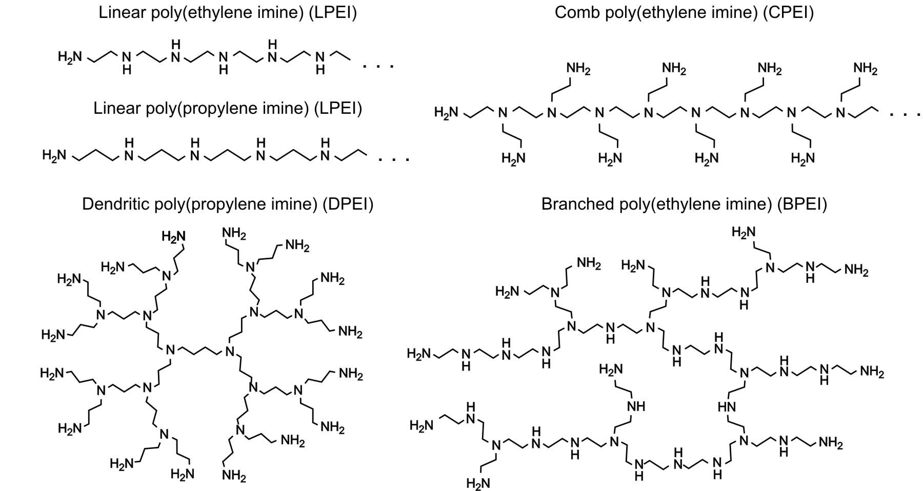
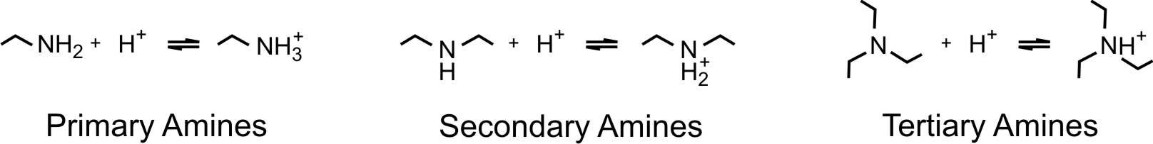
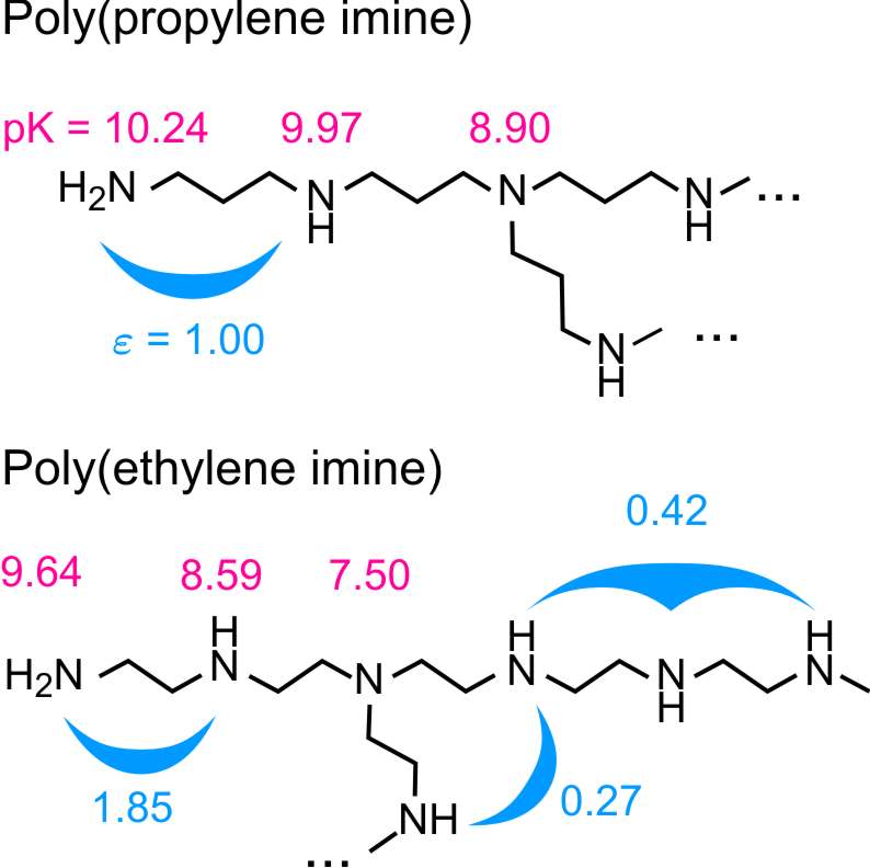
We will exemplify the situation with aliphatic polyamines as illustrated in the figure above. They may contain primary, secondary, and tertiary amine groups, each of which may protonate according to the reactions shown in the figure below.
There are many other types of weak polyelectrolytes, especially involving carboxylic groups, but these will not be discussed here in detail. Nevertheless, most principles discussed here apply to these polyelectrolytes too. The main complication one faces for many other polyelectrolytes, including poly(vinyl amine) or poly(acrylic acid), is their tacticity. The tacticity of a polymer leads to different isomeric structures, which may protonate in different ways. Poly(maleic acid) and poly(fumaric acid) differ only in their tacticity, and as a consequence, their protonation behavior differs substantially [1,2].
Proton binding isotherms can be measured by potentiometric titrations [2]. In such an experiment, one dissolves the acid or base in a solution, makes controlled small additions of a strong base or acid, and measures the solution pH after each addition. These binding isotherms are known for simple monoprotic or diprotic acids and bases, one usually makes no effort to obtain such binding isotherms, but one rather directly determines the binding constants. For weak polyelectrolytes, the situation is somewhat different, however. In that case, one can use a potentiometric titration to extract the amount of protons bound by the polyelectrolyte. Thereby, one must subtract the effect of the autoionization of water, and also take the dilution effect into account. Such experiments are nowadays carried out with computer controlled titration setups, and one can extract the proton binding isotherm [2]. The isotherm is normally represented as the degree of protonation θ versus pH. The titration curves of the aliphatic polyamines shown above have all been measured in this fashion.
Binding of protons to polyprotic molecules can be described with the site binding model [1,2]. This model assumes that each site can be in two states, namely deprotonated and protonated. To describe this situation mathematically, one introduces for each ionizable site i a state variable si, where si = 0 when the site is deprotonated and si = 1 when the site is protonated. The collection of all these variables s1, s2,... ,sN characterizes the protonation state of the entire molecule, whereby N is the number of ionizable sites. Each protonation state will have a different free energy, and one can express this free energy as a series expansion in the state variables si. Truncating this expansion to the quadratic order, we can obtain

where n = Σisi is the total number of protons bound, pKi is the microscopic protonation constant of the site i, εij is the pair interaction parameter between site i and site j, and the thermal energy is β-1 = kBT where kB is the Boltzmann constant, and T is the absolute temperature. The factor ln10 has been introduced to retain the relation to the pH scale. The binding isotherm can be obtained from a thermal average of the state variables
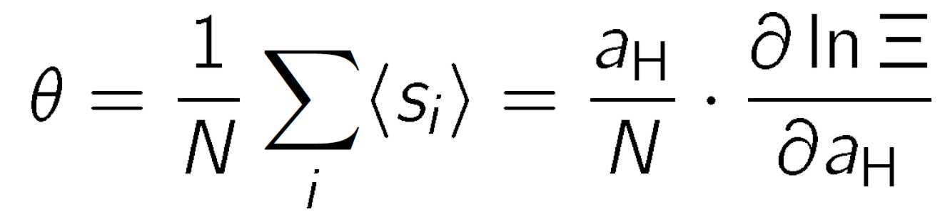
which can be obtained from the derivative of the semi-grand partition function
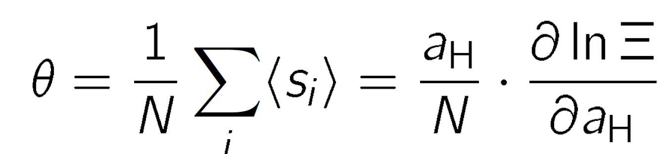
where aH is the activity of the protons and pH = - log aH. To evaluate the binding isotherm for a given molecule, one must specify the protonation constants and all interaction parameters. For poyelectrolytes, where N is very large, evaluation of the corresponding thermal averages can be computationally intensive.
When all sites are identical and non-interacting, the site binding model reduces to the Langmuir binding isotherm
![]()
where log K = pK. Each site protonates independently, in the same way as for a monoprotic acid or base. In the presence of interactions, the situation is more complex, but can be simplified somewhat when the interactions are short ranged. In that case, transfer matrix techniques can be used, which even may lead to explicit expressions of the isotherm. Otherwise, one can always resort to Monte Carlo simulation techniques to calculate the isotherm. The computational details are given in the literature [1,2]. One encounters short-range interactions in the case of protonation of polyelectrolytes. In the following, we will discuss two such models.
 Naive model: This model assumes that all sites independently have the same affinity for protons with a common protonation constant of pK = 10. Moreover, one assumes that only nearest neighbor interactions do not vanish, and that they can all be described with a common the pair interaction parameter ε = 2. These parameters roughly correspond to poly(ethylene imine).
Realistic model: This model uses a more accurate parameterization of poly(ethylene imine) and poly(propylene imine). The proton affinities of primary, secondary, and tertiary amines are assumed to be different. Moreover, longer ranged and higher order interaction parameters are introduced. Their numerical values are summarized in the figure on the left. They were estimated from ionization constants of small aliphatic polyamines, which feature the same structural units as the polyelectrolytes [2].
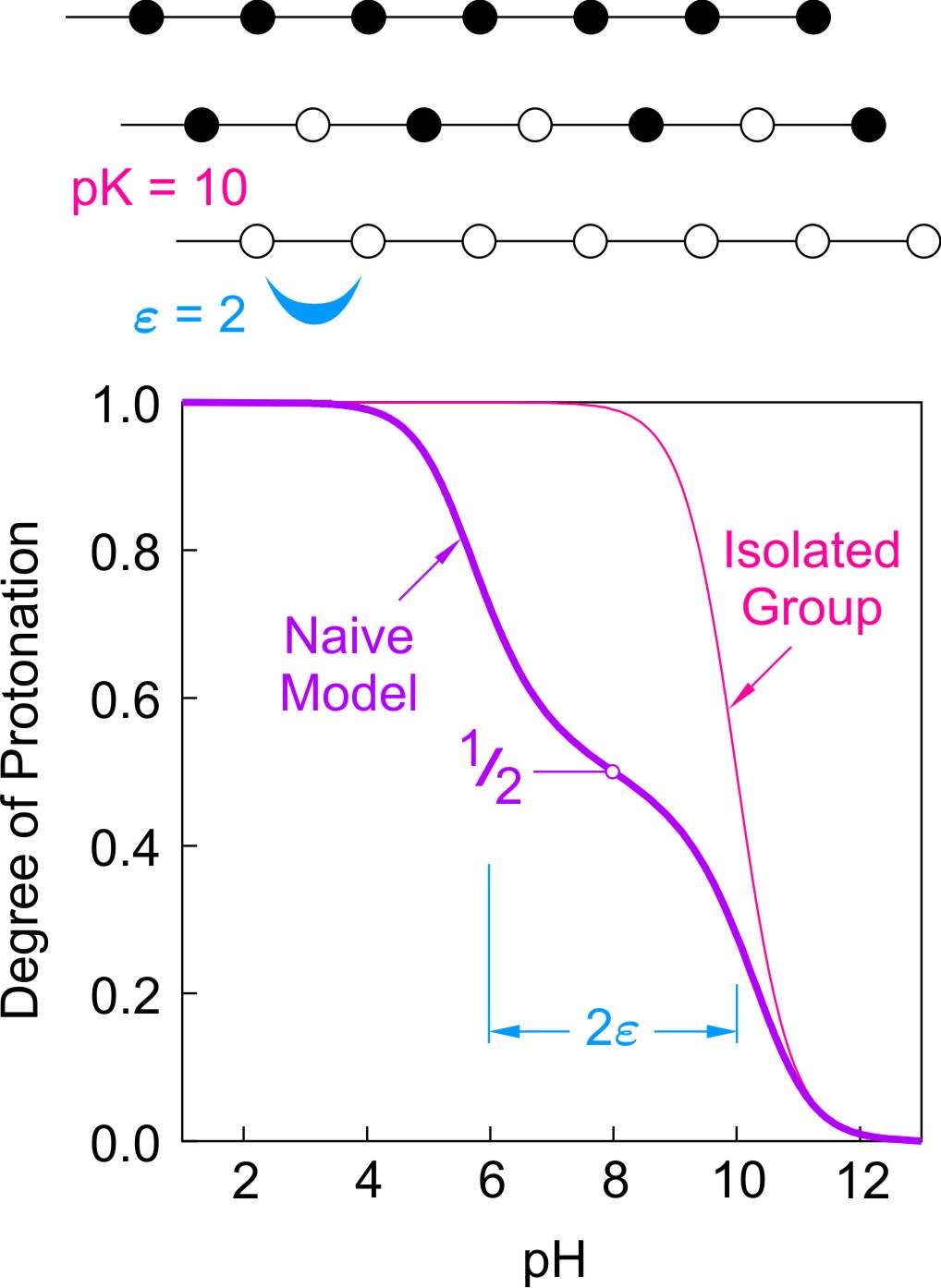
Let us first discuss the ionization of a linear polyelectrolyte. Each site has two nearest neighbors. The naive model assumes that the sites are arranged along a line and that only nearest neighbors interact. The right figure shows on the top the fully protonated and deprotonated molecule. The protonated sites are shown as full circles and the deprotonated ones as open ones. The end groups are unimportant for long chains. The predicted binding isotherm is shown in the lower part of the figure. One observes a typical two-step behavior with an intermediate plateau at θ = 1/2. This plateau is due to a stable intermediate microstate, where every second group is protonated. The stability of this state originates from the fact that the molecule minimizes its free energy by avoiding all nearest neighbor pair interactions. The first protonation step is situated at pH = 10, which corresponds to the protonation of the isolated sites. The second protonation step occurs at pH = 4. The splitting between the two steps corresponds to 2ε, since two pair interactions must be overcome to protonate a site in between two sites that are already protonated.
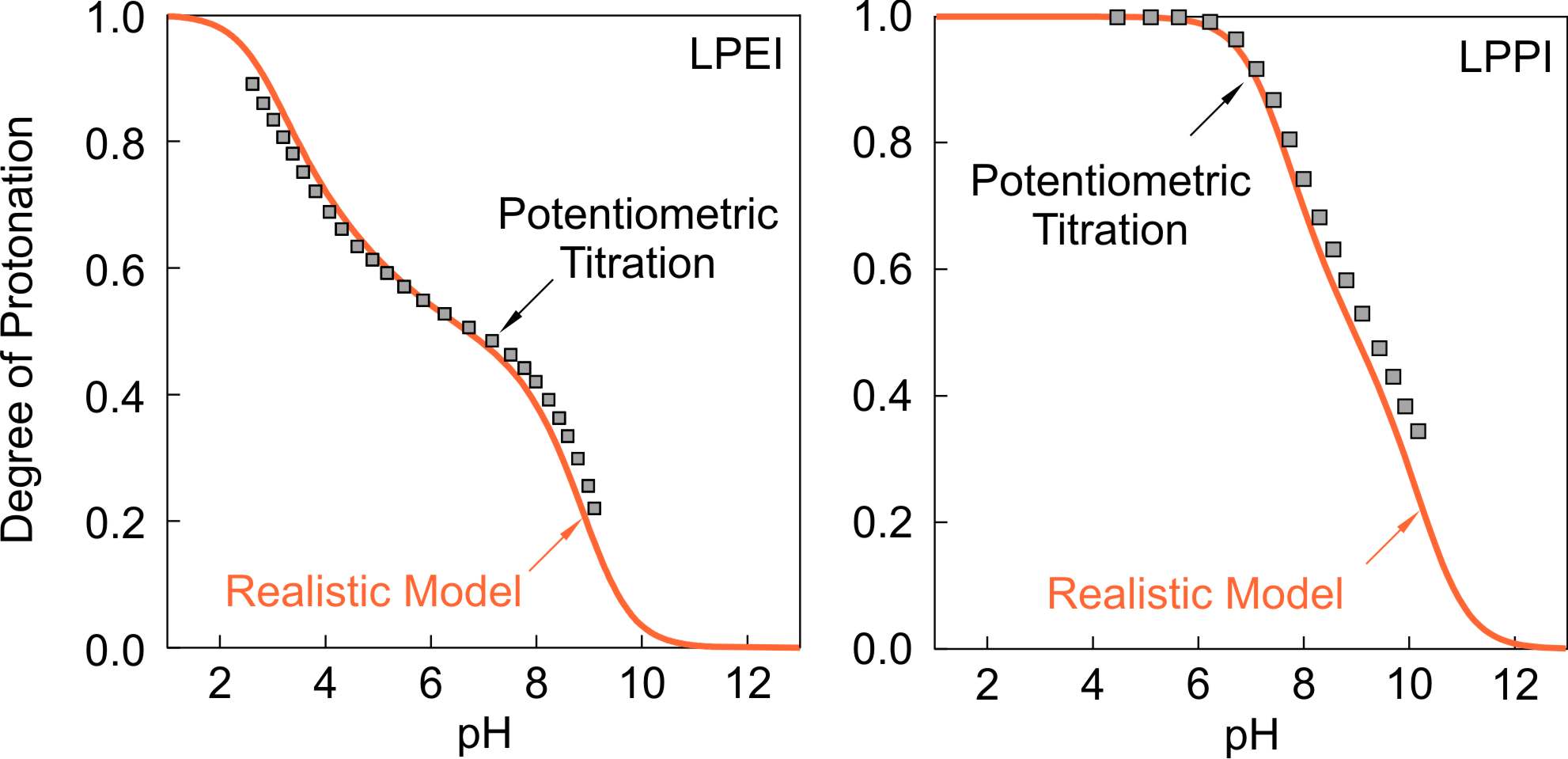 Experimental titration data for LPEI [3] and LPPI [4] are compared with predictions of the realistic model in the figure on the left. One observes that the experimental titration curves agree rather well with the realistic model. For LPEI the model introduces strong nearest neighbor interaction parameters between pairs of sites and between triplets.
The triplet interaction parameter is necessary to capture the asymmetry of the titration curve.
One observes that the experimental binding curve also shows the expected two step behavior.
The situation for LPPI is similar,
but the interactions are much weaker, and only pair interactions are present. In this case, the two step behavior is not well developed, and the presence of interactions only leads to a broadening of the binding curve. Such broadening has also been reported for other polyelectrolytes, where the ionizable groups are not too closely spaced.
Experimental titration data for LPEI [3] and LPPI [4] are compared with predictions of the realistic model in the figure on the left. One observes that the experimental titration curves agree rather well with the realistic model. For LPEI the model introduces strong nearest neighbor interaction parameters between pairs of sites and between triplets.
The triplet interaction parameter is necessary to capture the asymmetry of the titration curve.
One observes that the experimental binding curve also shows the expected two step behavior.
The situation for LPPI is similar,
but the interactions are much weaker, and only pair interactions are present. In this case, the two step behavior is not well developed, and the presence of interactions only leads to a broadening of the binding curve. Such broadening has also been reported for other polyelectrolytes, where the ionizable groups are not too closely spaced.
In this highly branched structure, each ionizable site in the interior has three nearest neighbors, and one neighbor on the rim. The prediction of the naive model is shown in the middle panel of the figure below. The curve again features an intermediate plateau. Now the plateau is situated at θ = 2/3. This value reflects the fraction of protonated sites in a stable microstate. In this microstate, the protonated sites are again arranged such that all nearest neighbor interactions are avoided. Thereby, the outermost sites are pronotated, and then the shell further inside remains deprotonated. The next shell is protonated again. Thus, the even shells are protonated, and the odd ones remain deprotonated. During the first protonation step, the isolated sites bind protons at pH = 10. In the second protonation step occuring at pH = 4, protons have to bind to sites with three nearest neighbors that are protonated. The splitting is therefore 3ε.
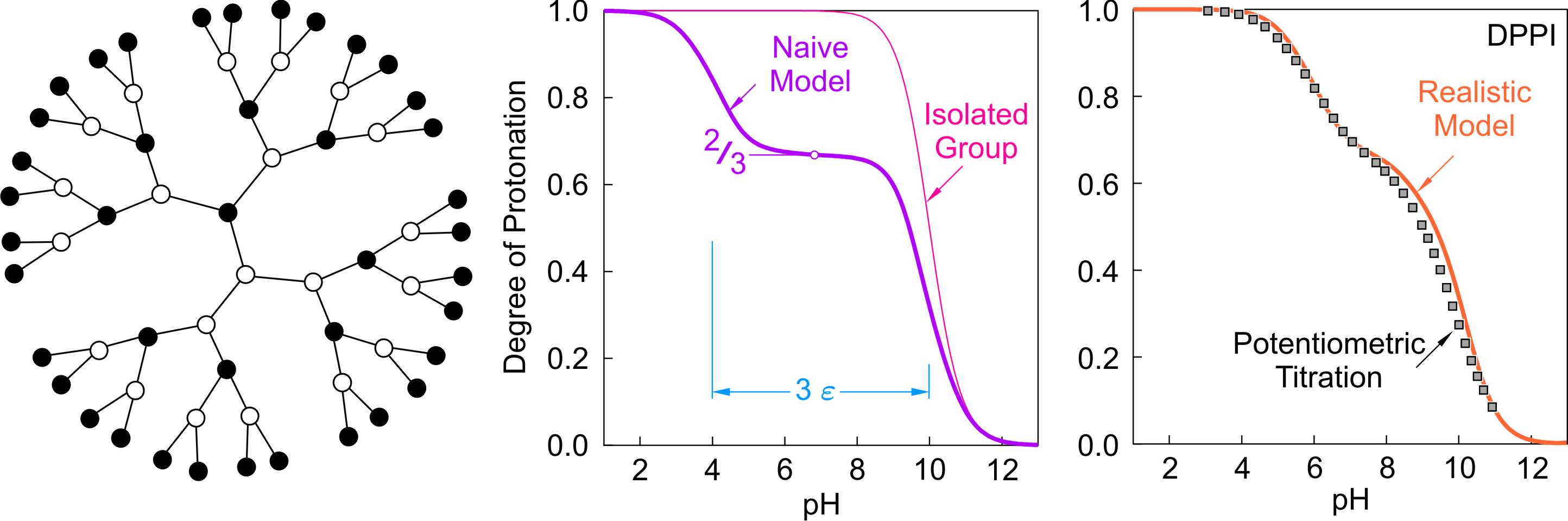
Dendritic poly(propylene imine) illustrates this behavior and is shown on the left in the figure above [5]. In this molecule, however, the nearest neighbor pair interactions are rather weak. Nevertheless, they show a clear two step protonation behavior with the intermeate plateau at θ = 2/3. The realistic model captures again the behavior well. Note that the curve is broadened, since the ionization constants of the primary and tertiary amines are not the same. The tertiary groups are more acidic than the primary ones.
The other relevant branched structure is the comb polyelectrolyte. The binding isotherm for the naive model is shown in the figure below. In this case, sites with three nearest neighbors are arranged along the backbone, and the side chains have only one neighbor. Thus structure protonates in three steps, and features two intermediate plateaus. The first plateau occurs at θ = 1/2. Thereby, only the side groups are protonated and the structure avoids all pair interactions. The second plateau is situated at θ = 3/4, and now also every second group along the backbone is protonated. The first protonation step occur at pH = 10 and again reflects the protonation of the isolated groups. During the second protonation step at pH = 8 one pair interaction must be overcome, and therefore the spacing is ε. In the last protonation step, which occurs at pH = 4, three pair interactions are relevant, and thus the splitting is 3ε.
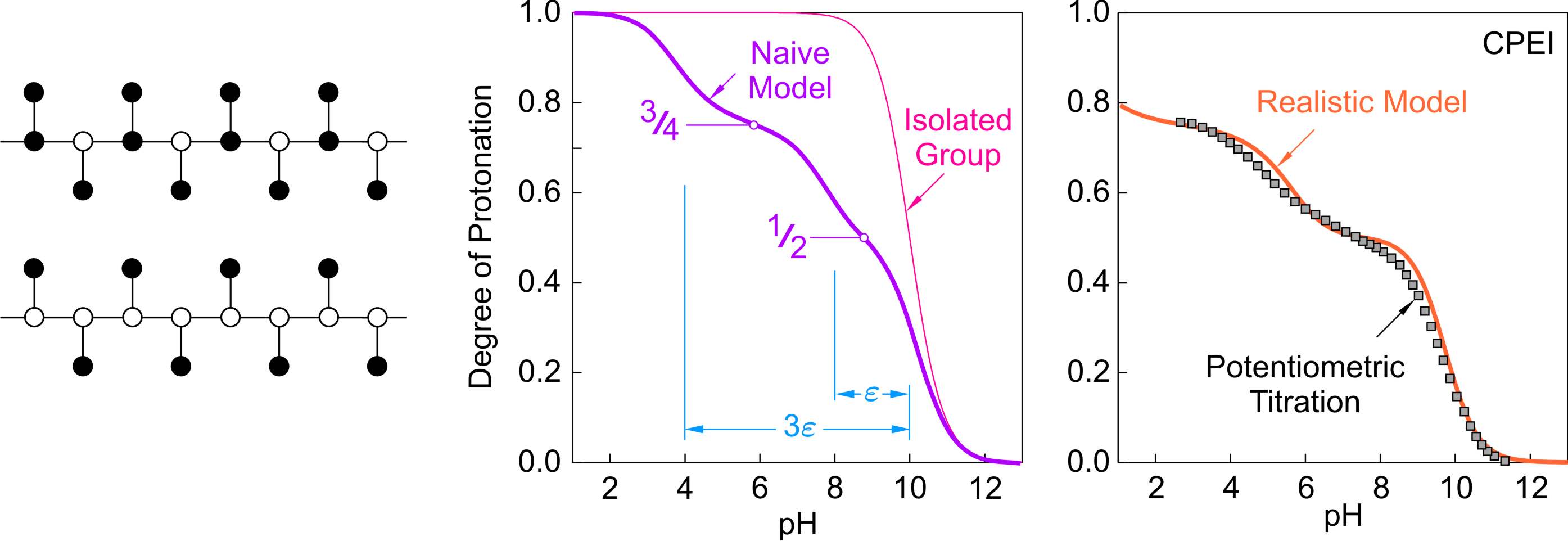
The experimental titration curve of CPEI is compared with the prediction of the realistic model in the figure above on the right [6]. Again, the model prediction is quite reasonable and shows the expected three step behavior. However, the role of the interactions is so strong, that the last protonation step could no longer be recorded in the titration experiment. This splitting is substantial for two reasons. Firstly, the tertiary amines are again more acidic than the primary ones. Secondly, the triplet interactions act between three different pairs of sites, and they also contribute to the splitting substantially.
The last structure to be discussed is a randomly branched polyelectrolyte. For simplicity, we assume that no ring structures are present and that sites with one, two, and three neighbors are roughly in the same proportions. The expected binding isotherm based on the naive model is shown in the middle of the figure below. There are no clearly developed intermediate steps. However, up to θ < 1/2 of the sites protonate independently, which lead to the rapid rise of the isotherm, and results in the intermediate structure shown. Further protonation of this structure can be thought to proceed in three different steps. In the first step, sites with one neighboring protonated group acquire a proton, and leads to a splitting of ε. In the second step, sites with two neighboring protonated groups acquire a proton, and lead to a splitting of 2ε. Finally, sites with three neighboring groups lead to a splitting of 3ε. Taking all these steps together, one obtains a rather featureless binding isotherm shown below.
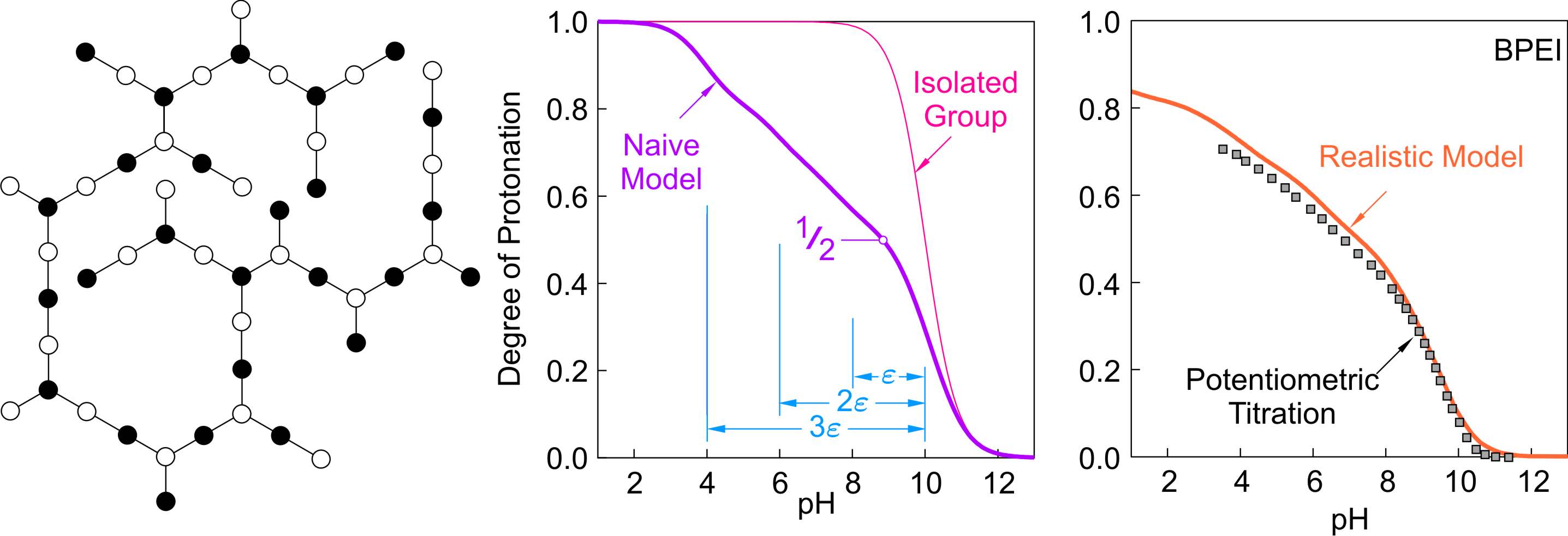
This structure is realized in BPEI [7]. The prediction of the binding curves with the realistic model leads to rather good agreement with the experiment as shown in the above figure on the right. The titration curve is broadened also at θ < 1/2 since the different amine groups have different affinities to protons. One observes again that BPEI does not fully protonate in the experimentally accessible pH window.
The site binding model is capable to capture the protonation behavior of various poly(ethylene imines) and poly(propylene imines). The main tenet of the model is that interactions between neighboring sites are taken into account, which leads to a binding isotherm that cannot be expressed in a simple algebraic form. For small molecules, on the other hand, the model reduces to the classical chemical equilibrium description of the protonation equilibria, whereby the corresponding binding constants are again influenced by the interactions between the sites. The model can be extended to other types of polyelectrolytes, although in many situations one must deal with their tacticity, which is often not known very precisely.
Michal Borkovec, Ger J. M. Koper
Email.
michal.borkovec@unige.ch, g.j.m.koper@tudelft.nl
www.colloid.ch/polyelectrolytes
First posted, September 15, 2013, last revision, September 6, 2014
This work is licensed under a Creative Commons Attribution 4.0 International License.
[1] Koper G. J. M., Borkovec M. (2010) Proton binding by linear, branched, and hyperbranched polyelectrolytes, Polymer, 51, 5649-5662, 10.1016/j.polymer.2010.08.067.
[2] Borkovec M., Jönsson B. and Koper G. J. M. (2001), Ionization processes and proton binding in polyprotic systems: Small molecules, proteins, interfaces and polyelectrolytes, Surf. Colloid Sci., 16, 99-339, ISBN 9780306464560.
[3] Smits R. G., Koper G. J. M., Mandel M. (1993) The influence of nearest-neighbor and next-nearest-neighbor interactions on the potentiometric titration of linear poly(ethylenimine), J. Phys. Chem., 97, 5745-5751, 10.1021/j100123a047.
[4] C. W. Schläpfer, University of Fribourg, private communication, 2002.
[5] van Duijvenbode R. C., Borkovec M., Koper G. J. M. (1998) Acid-base properties of poly(propylene imine) dendrimers, Polymer, 39, 2657-2664,10.1016/S0032-3861(97)00573-9.
[6] Koper G. J. M., van Duijvenbode R. C., Stam D. D. P. W., Steuerle U., Borkovec M. (2003) Synthesis and protonation behavior of comblike poly(ethyleneimine), Macromolecules 36, 2500-2507, 10.1021/ma020819s.
[7] Borkovec M., Koper G. J. M. (1997) Proton binding characteristics of branched polyelectrolytes, Macromolecules, 30, 2151-2158; 10.1021/ma961312i.